很多篮球迷对NBA球员的习惯出手位置感兴趣,想要得到如下的这种图:
经搜索发现网上已有相关资源,基本都来源于How to Create NBA Shot Charts in Python,但是现在按照这些教程都不能重现。
本文将介绍怎样具体可操作的用python的matplotlib包实现绘制NBA球员投篮出手位置图。
要做到这件事主要是解决两个大问题:
- NBA球员的投篮数据从哪里获得 (大多网上已有资源卡在了这里)
- 怎么样绘制到图表
我们将练习到如下知识:
- 怎么样通过网页分析获取数据API
- 获取网页数据的基础方式
- 绘制篮球半场图
第一部分--获取球员投篮位置数据
NBA官方并没有提供公共的API方便我们访问球员的shot log, Web Scraping 201: finding the API这篇文章为我们提供了分析网页寻找数据API的方法,我们要分析NBA球员shot log可拆解成以下步骤:
- 锁定目标网站(哪个网站有NBA球员shot log数据)
- 具体网页对象(具体哪个网页有shot log数据)
- 分析shot log API
- 通过API获取感兴趣球员的shot log数据
1.锁定目标网站
目标网站:stats.nba.com
2.具体网页对象
shot log所在的页面标签可能会有改变,有时不在很显眼的位置,这也是很多教程失效的原因(只给了最后API的网址,没有说这个网址是怎么来的),所以这个得花时间找一下。
首先打开目标网站stats.nba.com,按下图所示依次点击Player,See All Stats
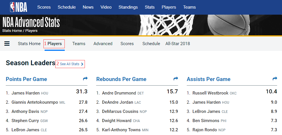
按照图中1、2顺序点击后会得到以下页面
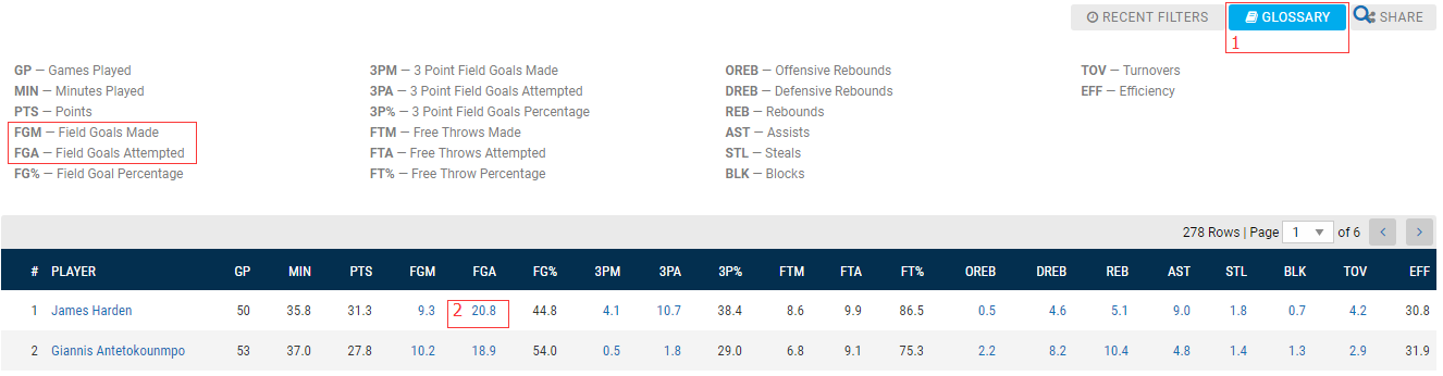
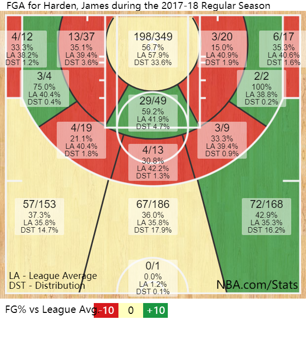
页面表格是每个NBA球员的数据,表头都是简写,通过图示点击GLOSSARY我们得到表头详细信息,其中FGA-Field Goals Attempted表示尝试投篮的位置,表格中每个球员的FGA列的数字都是可点击的,我们按上图所示点击James Harden的FGA列数字,跳转的结果是显示了James Harden2017-18常规赛的Hex Hap
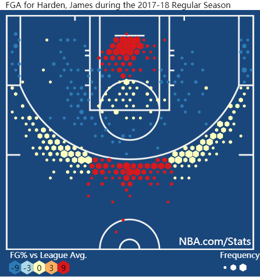
Shot Plot
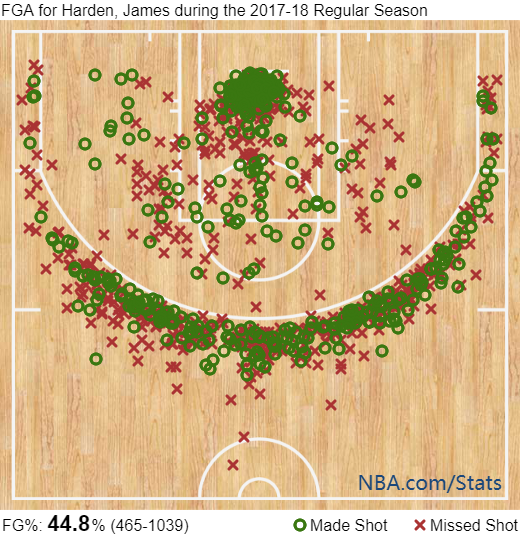
Shot Zones
好了,可以结束了...
等等,我们的目的不是简单得到Shot Plot,而是要练习一些知识,所以,继续
点击James Harden的FGA数据,跳转后的页面除了以上3个图还包括以下这个表格
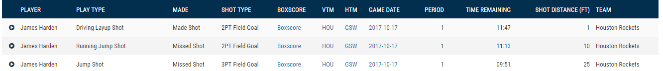
这个表格的内容结合Shot Plot的图,可以确定,要找的具体网页对象应该是这个页面了,但是表格中并没有直接给出投篮位置信息,这个网页访问的API应该包括这些信息,所以我们进入下面的步骤
3.分析shot log API
我们以Chrome浏览器为例,在上一步找到的具体网页对象页面打开浏览器的开发者选项(更多工具->开发者工具),然后按F5键,刷新页面,你将得到如下页面
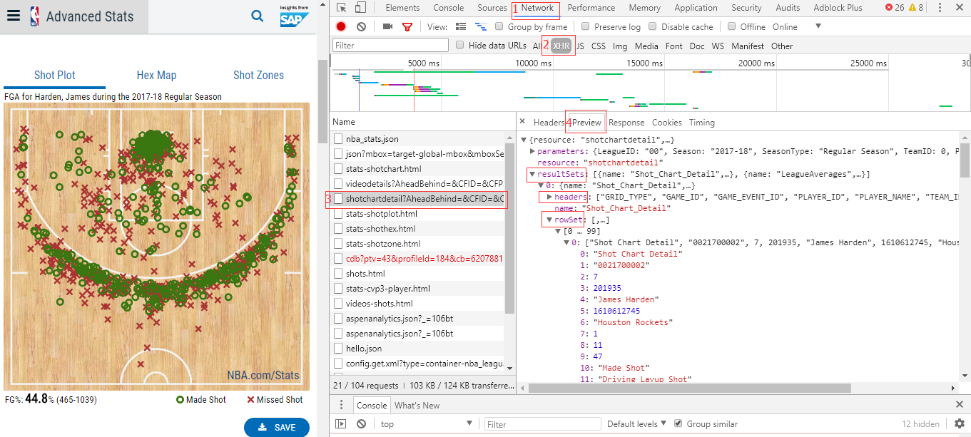
我们按上图红色数字标注,依次点击,选择Network,然后点击XHR进行过滤,XHR是XMLHttpRequest的简写 - 这是一种用来获取XML或JSON数据的请求类型。经XHR筛选后表格中的有几个条目,红色数字标注为3的既是我们将要查找的shot log API,Preview标签中包括:
- resource - 请求的名称 shotchartdetail。
- parameters - 请求参数,提交给API的请求参数,我们可以理解成SQL语言的条件语句,例如赛季、球员ID等等,我们改变URL中的参数就能得到不同的数据
- resultSets - 请求得到的数据集,包含两个表格。仔细看表头(headers)第一个表格包含我们想要的shot log信息(LOC_X,LOC_Y)。
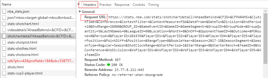
与Preview并列的Headers标签包含:
- Request URL - API URL
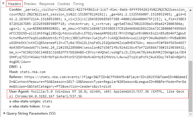
- Requset Headers - 请的表头,用程序爬取网页请求数据时会用到
通过API获取感兴趣球员的shot log数据
4.通过API获取感兴趣球员的shot log数据
上一步得到了James Hardenshot log的Request URL和Requset Headers,下面我们要做的是通过python代码获取shot log数据,以下是代码
    import requests
    import pandas as pd

    shot_chart_url = 'http://stats.nba.com/stats/shotchartdetail?AheadBehind=&'\
                     'CFID=&CFPARAMS=&ClutchTime=&Conference=&ContextFilter=&ContextMeasure=FGA'\
                     '&DateFrom=&DateTo=&Division=&EndPeriod=10&EndRange=28800&GROUP_ID=&GameEventID='\
                     '&GameID=&GameSegment=&GroupID=&GroupMode=&GroupQuantity=5&LastNGames=0&LeagueID=00'\
                     '&Location=&Month=0&OnOff=&OpponentTeamID=0&Outcome=&PORound=0&Period=0&PlayerID={PlayerID}'\
                     '&PlayerID1=&PlayerID2=&PlayerID3=&PlayerID4=&PlayerID5=&PlayerPosition=&PointDiff=&Position='\
                     '&RangeType=0&RookieYear=&Season={Season}&SeasonSegment=&SeasonType={SeasonType}'\
                     '&ShotClockRange=&StartPeriod=1&StartRange=0&StarterBench=&TeamID=0&VsConference='\
                     '&VsDivision=&VsPlayerID1=&VsPlayerID2=&VsPlayerID3=&VsPlayerID4=&VsPlayerID5='\
                     '&VsTeamID='.format(PlayerID=201935,Season='2017-18',SeasonType='Regular+Season')

    header = { 'User-Agent' : 'Mozilla/5.0 (Windows NT 6.1; Win64; x64) AppleWebKit/537.36 (KHTML, like Gecko)'\
                              ' Chrome/62.0.3202.94 Safari/537.36'}

    response = requests.get(shot_chart_url,headers=header)
    # headers是模拟浏览器访问行为,现在没有这一项获取不到数据

    headers = response.json()['resultSets'][0]['headers']
    shots = response.json()['resultSets'][0]['rowSet']
    shot_df = pd.DataFrame(shots, columns=headers)

    # View the head of the DataFrame and all its columns
    from IPython.display import display
    with pd.option_context('display.max_columns', None):
        display(shot_df.head())
    # Or
    #shot_df.head().to_excel('outfile.xls',index=True,header=True)
我们得到的pandas DataFrame:shot_df,表头及前3行数据展示如下:

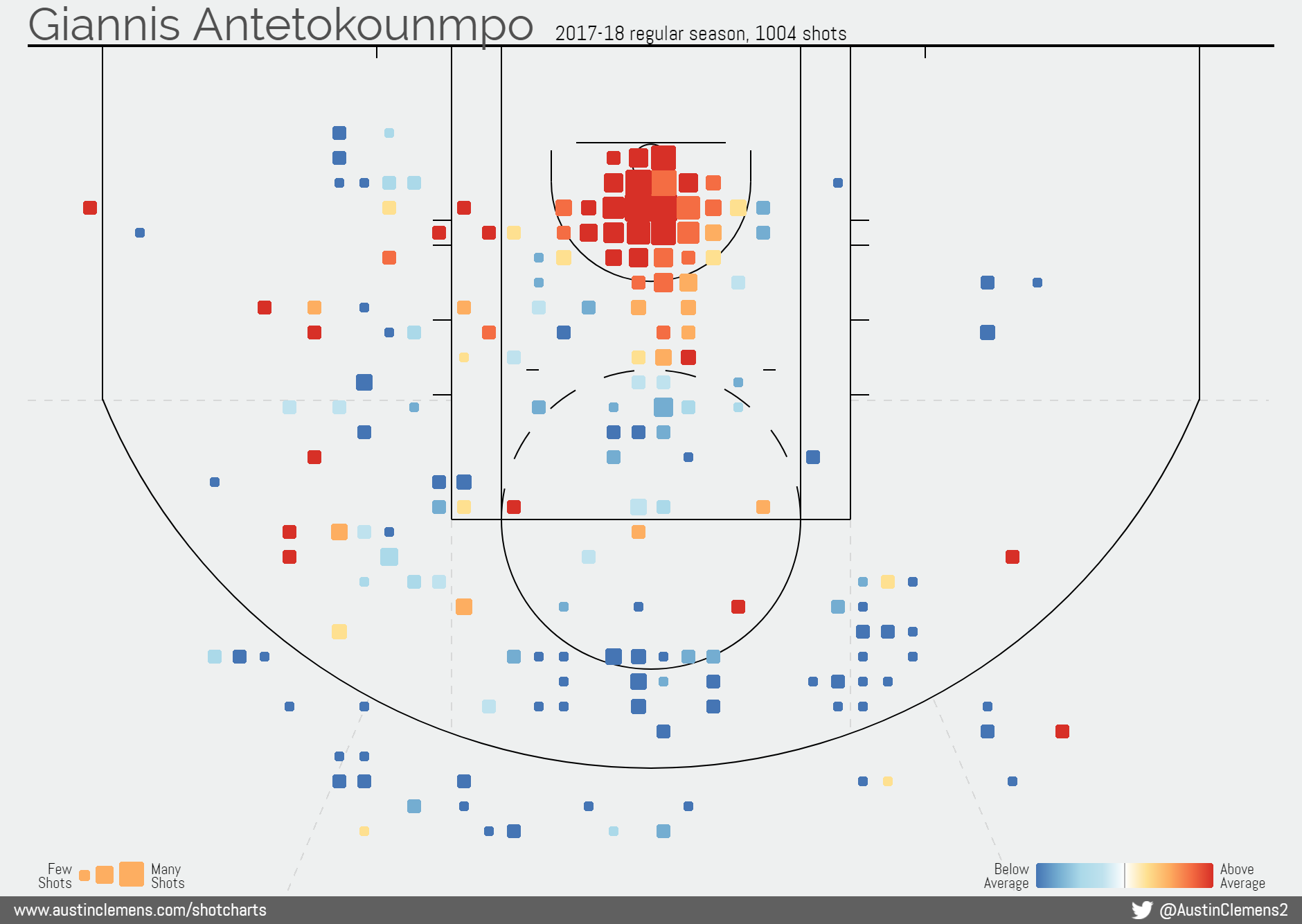
shot_chart_url其中PlayerID、Season、SeasonType三项是可变参数,如果想获得其他球员的PlayerID可以登录nba.com/players搜索感兴趣球员的名字,如下
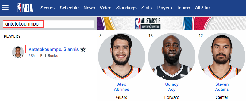
点击搜索结果,跳转到页面的网址最后一项既是PlayerID,例如:http://www.nba.com/players/giannis/antetokounmpo/203507中的203507即是字母哥的PlayerID。
我们这一步得到的shot_df包含了James Harden在2017-18赛季常规赛目前为止(20180219全明星赛)所有投篮尝试。我们需要的数据为LOC_X和LOC_Y两列,这些是每次投篮尝试的坐标值,然后可以将这些坐标值绘制到代表篮球场的坐标轴上,当然我们可能还需要EVENT_TYPE列,来区分投篮是否投进。
第二部分--绘制球员shot log到球场图
关于这一部分,How to Create NBA Shot Charts in Python已经做了非常优秀的工作,我们会延续其框架,并对代码做少许修改以达到更好的适用性。
首先我们对上一步得到的James Harden的shot log LOC_X和LOC_Y进行快速绘图,看其X、Y是怎么定义的。
import matplotlib.pyplot as plt

fig = plt.figure(figsize=(4.3,4))
ax = fig.add_subplot(111)
ax.scatter(shot_df.LOC_X, shot_df.LOC_Y)
plt.show()
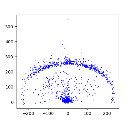
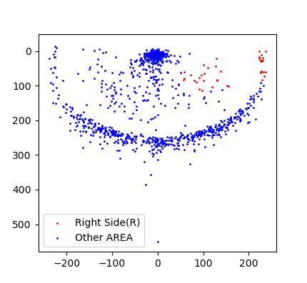
通过快速预览图我们对LOC_X和LOC_Y有了一个大概的认识,有一点需要注意:LOC_X其实是观众视野从中场面向篮筐来说的,LOC_X是正值则在篮筐的左边。所以最终绘图时需要按以下代码做调整,我们以shot log中Right Side(R) 投篮区域(投篮区域划分请参考前文Shot Zones图)的出手作为示例说明。
right_shot_df = shot_df[shot_df.SHOT_ZONE_AREA == "Right Side(R)"]
other_shot_df = shot_df[~(shot_df.SHOT_ZONE_AREA == "Right Side(R)")]

fig = plt.figure(figsize=(4.3,4))
ax = fig.add_subplot(111)
ax.scatter(right_shot_df.LOC_X, right_shot_df.LOC_Y, s=1, c='red', label='Right Side(R)')
ax.scatter(other_shot_df.LOC_X, other_shot_df.LOC_Y, s=1, c='blue', label='Other AREA')
ax.set_ylim(top=-50,bottom=580)
ax.legend()
plt.show()
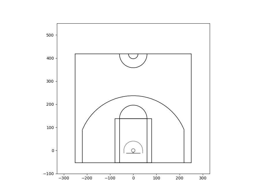
画篮球半场图
通过对LOC_X和LOC_Y数据的快速画图,我们大概知道了篮筐的位置大概就是LOC_X和LOC_Y的原点。知道了这一点,我们结合篮球半场的具体尺寸 (下图)和比例就可以画出篮球半场图了。

通过上图我们知道了篮球场宽度是50FT,转换成INCH是600IN,篮球场长94FT,转换成INCH是1128IN,再结合我们上一步画出的投篮点快速预览图,通过对很多球员的LOC_Y为0时,LOC_X与SHOT_DISTANCE,我们能够推测出LOC_X和LOC_Y的单位与IN的换算大概为10/12。
画图函数如下:
import matplotlib.pyplot as plt
from matplotlib.patches import Rectangle, Arc,Wedge

class data_linewidth_plot():
    def __init__(self,**kwargs):
        self.ax = kwargs.pop("ax", plt.gca())
        self.lw_data = kwargs.pop("linewidth", 1)
        self.lw = 1
        #self.ax.figure.canvas.draw()
        self.ppd=72./fig.dpi
        self.trans = self.ax.transData.transform
        self._resize()

    def _resize(self):
        lw =  ((self.trans((1,self.lw_data))-self.trans((0,0)))*self.ppd)[1]
        self.lw = lw

def draw_half_court(ax=None, unit=1):
    lw = unit * 2 #line width
    color = 'k'
    # 精确line width
    court_lw = data_linewidth_plot(ax = ax,linewidth = lw).lw

    ## Create the basketball hoop
    #篮筐直径(内径)是18IN.,我们设置半径为9.2IN刨除line width 0.2IN,正好为篮筐半径
    hoop = Wedge((0, 0), unit * 9.2, 0, 360, width=unit * 0.2, color='#767676')
    hoop_neck = Rectangle((unit * -2, unit * -15 ), unit * 4, unit * 6, linewidth=None, color='#767676')

    ## Create backboard
    #Rectangle, left lower at xy = (x, y) with specified width, height and rotation angle
    backboard = Rectangle((unit * -36, unit * -15 ), unit * 72, court_lw, linewidth=None, color='#767676')
    # List of the court elements to be plotted onto the axes

    ## Restricted Zone, it is an arc with 4ft radius from center of the hoop
    restricted = Arc((0, 0), 96*unit+court_lw, 96*unit+court_lw, theta1=0, theta2=180,linewidth=court_lw, color='#767676', fill=False)
    restricted_left = Rectangle((-48*unit-court_lw/2, unit * -15 ), 0, unit * 17, linewidth=court_lw, color='#767676')
    restricted_right = Rectangle((unit*48+court_lw/2, unit * -15 ), 0, unit * 17, linewidth=court_lw, color='#767676')

    # Create free throw top arc  罚球线弧顶
    top_arc_diameter = 6 * 12 * 2*unit - court_lw
    top_free_throw = Arc((0, unit * 164), top_arc_diameter, top_arc_diameter, theta1=0, theta2=180,linewidth=court_lw, color=color, fill=False)
    # Create free throw bottom arc 罚球底弧
    bottom_free_throw = Arc((0, unit * 164), top_arc_diameter, top_arc_diameter, theta1=180, theta2=0,linewidth=abs(court_lw), color=color, linestyle='dashed', fill=False)
    # Create the outer box 0f the paint, width=16ft outside , height=18ft 10in
    outer_box = Rectangle((court_lw/2 - unit*96, -court_lw/2 - unit*63), 192*unit-court_lw, 230*unit-court_lw, linewidth=court_lw, color=color, fill=False)
    # Create the inner box of the paint, widt=12ft, height=height=18ft 10in
    inner_box = Rectangle((court_lw/2 - unit*72, -court_lw/2 - unit*63), 144*unit-court_lw, 230*unit-court_lw, linewidth=court_lw, color=color, fill=False)

    ## Three point line
    # Create the side 3pt lines, they are 14ft long before they begin to arc
    corner_three_left = Rectangle((-264*unit+court_lw/2, -63*unit-court_lw/2), 0, 14*12*unit +court_lw, linewidth=court_lw, color=color)
    corner_three_right = Rectangle((264*unit-court_lw/2, -63*unit-court_lw/2), 0, 14*12*unit +court_lw, linewidth=court_lw, color=color)
    # 3pt arc - center of arc will be the hoop, arc is 23'9" away from hoop
    # I just played around with the theta values until they lined up with the
    # threes
    three_diameter = (23 * 12 + 9) * 2*unit - court_lw
    three_arc = Arc((0, 0), three_diameter, three_diameter, theta1=21.9, theta2=158, linewidth=court_lw, color=color)

    # Center Court
    center_outer_arc = Arc((0, (94*12/2-63)*unit), 48*unit+court_lw, 48*unit+court_lw, theta1=180, theta2=0,linewidth=court_lw, color=color)
    center_inner_arc = Arc((0, (94*12/2-63)*unit), 144*unit-court_lw, 144*unit-court_lw, theta1=180, theta2=0,linewidth=court_lw, color=color)

    # Draw the half court line, baseline and side out bound lines
    outer_lines = Rectangle((-25*12*unit - court_lw/2, -63*unit-court_lw/2), 50*12*unit+court_lw, 94/2*12*unit + court_lw, linewidth=court_lw, color=color, fill=False)

    #2 IN. WIDE BY 3 FT. DEEP, 28 FT. INSIDE, 3FT. extenf onto court

    court_elements = [hoop_neck, backboard, restricted, restricted_left, restricted_right,top_free_throw,bottom_free_throw,
                        outer_box,inner_box, corner_three_left,corner_three_right,three_arc,center_outer_arc,center_inner_arc,outer_lines]

    # Add the court elements onto the axes
    for element in court_elements:
        ax.add_patch(element)
画图:
fig = plt.figure(figsize=(9,9))
ax = fig.add_subplot(111,aspect='equal')
ax.set_xlim(-330,330)
ax.set_ylim(-200,600)

draw_half_court(ax=ax)

plt.show()
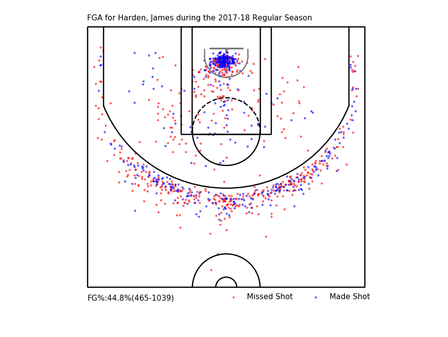
添加上投篮数据
fig = plt.figure(figsize=(9,8))
ax = fig.add_subplot(111,aspect='equal')
ax.set_xlim(-330,330)
ax.set_ylim(top= -100,bottom = 500)

draw_half_court(ax=ax,unit=10/12)

df_missed = shot_df[shot_df.EVENT_TYPE=='Missed Shot'][['LOC_X','LOC_Y']]
ax.scatter(df_missed.LOC_X, df_missed.LOC_Y,s=2,color='r',label = 'Missed Shot',alpha=0.5)
df_made = shot_df[shot_df.EVENT_TYPE=='Made Shot'][['LOC_X','LOC_Y']]
ax.scatter(df_made.LOC_X, df_made.LOC_Y,s=2,color='b',label = 'Made Shot',alpha=0.5)

legend = ax.legend(bbox_to_anchor=(0.49, 0.13), loc=2, borderaxespad=0.,prop={'size':8},ncol=2,frameon=False)
plt.axis('off')

FG = "%.1f" % ((df_made.shape[0]/shot_df.shape[0])*100)
ax.text(-250,440,'FG%:{0}%({1}-{2})'.format(FG,df_made.shape[0],shot_df.shape[0]), fontsize=8)
ax.text(-250,-63,'FGA for Harden, James during the 2017-18 Regular Season'.format(FG,df_made.shape[0],shot_df.shape[0]), fontsize=8)

plt.show()